Correlation
Next, you want to test the relationship with other (pseudo-metric) variables. In Learning Block 3, you have already learned about pairs.panel() from the library psych and corrplot() from the library corrplot. Now, instead of using the library psych, we will first create a plot using the library GGally, as it follows the same logic as all ggplots. For this, you will use the function ggpairs().
A plot with ggpairs() is structured the same way as a plot from pairs.panel():
 It is a matrix representation. There is a lower third
 lower, an upper third upper, and a diagonal diag. For each of these parts, you can set settings based on whether the pair of values in the cell of the matrix are both continuous variables (continuous), both discrete variables (discrete), or a combination (combo).
Before you start the challenge, a brief introduction to GGally. You can simply use the function ggpairs() from the library.
install.packages("GGally")
library("GGally")
Creating a Pairs Panel is easy with the function ggpairs(): The first argument is the dataset, and in the columns argument, you can restrict the selection to specific variables. Here, start with stfdem, agea, and gndr. Yes, you can also include categorical variables!
ggpairs(
  pss,
  columns = c(
    "stfdem",
    "agea",
    "gndr"
    )
)
## Warning: Removed 95 rows containing non-finite outside the scale range
## (`stat_density()`).## Warning in ggally_statistic(data = data, mapping = mapping, na.rm = na.rm, :
## Removed 249 rows containing missing values## Warning: Removed 95 rows containing non-finite outside the scale range
## (`stat_boxplot()`).## Warning: Removed 249 rows containing missing values or values outside the scale range
## (`geom_point()`).## Warning: Removed 157 rows containing non-finite outside the scale range
## (`stat_density()`).## Warning: Removed 157 rows containing non-finite outside the scale range
## (`stat_boxplot()`).## Warning: Removed 95 rows containing non-finite outside the scale range
## (`stat_bin()`).## Warning: Removed 157 rows containing non-finite outside the scale range
## (`stat_bin()`).
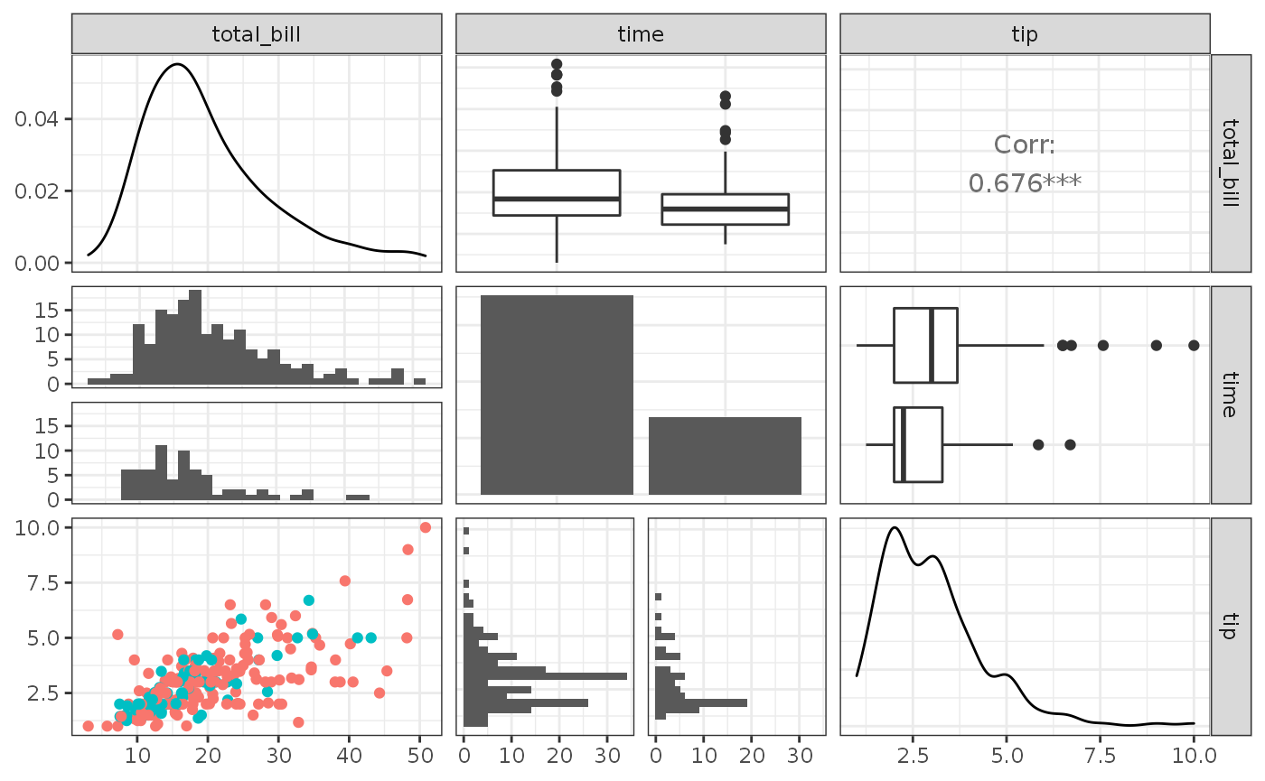
This will give you the default settings of the plot. In the diagonal, the density is displayed if the variable is continuous or a bar plot if the variable is discrete. In the upper third, if both variables are continuous, the correlation is shown. If a combination is present (i.e., one variable is continuous, the other is discrete), you will see a box plot. If both variables are discrete (not applicable here), the grouped frequencies are simply displayed in a bar chart. This way, you get a direct overview of the variables.
It is also possible to customize the individual areas: Let’s start with lower because we want to change the binwidth. In the lower argument, we name a list: it includes what we specifically want to display on continuous, combo, or discrete. If you want to make changes to the display, you need to wrap them in the wrap() function and within that, you can make changes as with normal ggplots. We now specify that for continuous pairs, a scatter plot should be displayed (points) and for mixed pairs (continuous - discrete), histograms in a facet (facethist), where we set the binwidth to \(1\). Additionally, we specify that the color should vary according to the category of the variable gndr (mapping = aes(color = gndr)).
ggpairs(
  pss,
  columns = c(
    "stfdem",
    "agea",
    "gndr"
    ),
  lower = list(
    continuous = "points",
    combo = wrap(
      "facethist",
      binwidth = 1
      ),
    mapping = aes(color = gndr)
  )
)
## Warning: Removed 95 rows containing non-finite outside the scale range
## (`stat_density()`).## Warning in ggally_statistic(data = data, mapping = mapping, na.rm = na.rm, :
## Removed 249 rows containing missing values## Warning: Removed 95 rows containing non-finite outside the scale range
## (`stat_boxplot()`).## Warning: Removed 249 rows containing missing values or values outside the scale range
## (`geom_point()`).## Warning: Removed 157 rows containing non-finite outside the scale range
## (`stat_density()`).## Warning: Removed 157 rows containing non-finite outside the scale range
## (`stat_boxplot()`).## Warning: Removed 95 rows containing non-finite outside the scale range
## (`stat_bin()`).## Warning: Removed 157 rows containing non-finite outside the scale range
## (`stat_bin()`).
We see that the scatter plot is not quite optimal yet, as one variable is pseudo-metric again. Therefore, we add jitter:
ggpairs(
  pss,
  columns = c(
    "stfdem",
    "agea",
    "gndr"
    ),
  lower = list(
    continuous = wrap(
      "points",
      position = position_jitter(width = 0.5)
    ),
    combo = wrap(
      "facethist",
      binwidth = 1
      ),
    mapping = aes(color = gndr)
  )
)
## Warning: Removed 95 rows containing non-finite outside the scale range
## (`stat_density()`).## Warning in ggally_statistic(data = data, mapping = mapping, na.rm = na.rm, :
## Removed 249 rows containing missing values## Warning: Removed 95 rows containing non-finite outside the scale range
## (`stat_boxplot()`).## Warning: Removed 249 rows containing missing values or values outside the scale range
## (`geom_point()`).## Warning: Removed 157 rows containing non-finite outside the scale range
## (`stat_density()`).## Warning: Removed 157 rows containing non-finite outside the scale range
## (`stat_boxplot()`).## Warning: Removed 95 rows containing non-finite outside the scale range
## (`stat_bin()`).## Warning: Removed 157 rows containing non-finite outside the scale range
## (`stat_bin()`).
Now the whole thing looks better and indicates that we probably do not have a correlation between age and satisfaction with democracy.
Next, we adjust the upper third upper. We specify that the correlation should be displayed for continuous pairs and a box plot for combo pairs. We also specify again that the colors should be different based on gender.
ggpairs(
  pss,
  columns = c(
    "stfdem",
    "agea",
    "gndr"
    ),
  lower = list(
    continuous = wrap(
      "points",
      position = position_jitter(width = 0.5)
    ),
    combo = wrap(
      "facethist",
      binwidth = 1
      ),
    mapping = aes(color = gndr)
  ),
  upper = list(
    continuous = "cor",
    combo = "box_no_facet",
    mapping = aes(color = gndr)
  )
)
## Warning: Removed 95 rows containing non-finite outside the scale range
## (`stat_density()`).## Warning in ggally_statistic(data = data, mapping = mapping, na.rm = na.rm, :
## Removed 249 rows containing missing values## Warning: Removed 95 rows containing non-finite outside the scale range
## (`stat_boxplot()`).## Warning: Removed 249 rows containing missing values or values outside the scale range
## (`geom_point()`).## Warning: Removed 157 rows containing non-finite outside the scale range
## (`stat_density()`).## Warning: Removed 157 rows containing non-finite outside the scale range
## (`stat_boxplot()`).## Warning: Removed 95 rows containing non-finite outside the scale range
## (`stat_bin()`).## Warning: Removed 157 rows containing non-finite outside the scale range
## (`stat_bin()`).
There are good display options for continuous in both lower and upper (a complete overview can be found here):
pointscordensitysmooth/smooth_lm
For combo in both lower and upper, the following recommended display options are available:
- box_no_facet / box
- facethist
Next, we want to adjust the diagonal!
pp1 <- ggpairs(
  pss,
  columns = c(
    "stfdem",
    "agea",
    "gndr"
    ),
  lower = list(
    continuous = wrap(
      "points",
      position = position_jitter(width = 0.5)
    ),
    combo = wrap(
      "facethist",
      binwidth = 1
      ),
    mapping = aes(color = gndr)
  ),
  upper = list(
    continuous = "cor",
    combo = "box_no_facet",
    mapping = aes(color = gndr)
  ),
  diag = list(
    continuous = wrap("densityDiag", bw = 1),
    discrete = "barDiag",
    mapping = aes(
      color = gndr,
      alpha = 1
    )
  )
)

pp1
## Warning: Removed 95 rows containing non-finite outside the scale range
## (`stat_density()`).## Warning in ggally_statistic(data = data, mapping = mapping, na.rm = na.rm, :
## Removed 249 rows containing missing values## Warning: Removed 95 rows containing non-finite outside the scale range
## (`stat_boxplot()`).## Warning: Removed 249 rows containing missing values or values outside the scale range
## (`geom_point()`).## Warning: Removed 157 rows containing non-finite outside the scale range
## (`stat_density()`).## Warning: Removed 157 rows containing non-finite outside the scale range
## (`stat_boxplot()`).## Warning: Removed 95 rows containing non-finite outside the scale range
## (`stat_bin()`).## Warning: Removed 157 rows containing non-finite outside the scale range
## (`stat_bin()`).
There are fewer options in the diag argument:
barDiagdensityDiagblankDiag(diagonal is empty)
Simply try something out in the code and experiment with the available options.
Lastly, we want to adjust the colors here and again use the library beyonce: Remember, you can manually adjust the colors using scale_color_manual() or scale_fill_manual()!
library("beyonce")

pp1 +
  scale_color_manual(values = beyonce_palette(72)) +
  scale_fill_manual(values = beyonce_palette(72))
## Warning in ggally_statistic(data = data, mapping = mapping, na.rm = na.rm, :
## Removed 249 rows containing missing values## Warning: Removed 95 rows containing non-finite outside the scale range
## (`stat_density()`).## Warning: Removed 95 rows containing non-finite outside the scale range
## (`stat_boxplot()`).## Warning: Removed 249 rows containing missing values or values outside the scale range
## (`geom_point()`).## Warning: Removed 157 rows containing non-finite outside the scale range
## (`stat_density()`).## Warning: Removed 157 rows containing non-finite outside the scale range
## (`stat_boxplot()`).## Warning: Removed 95 rows containing non-finite outside the scale range
## (`stat_bin()`).## Warning: Removed 157 rows containing non-finite outside the scale range
## (`stat_bin()`).
On the next page, we’ll move on to the challenge!