Fundamentals of Linear Regression
With linear regression, we estimate the causal relationship between one (or more) independent variable(s) and a dependent variable. The model is typically estimated using the Ordinary Least Squares (OLS) method, giving us the Best Linear Unbiased Estimator (BLUE). This holds true only under certain assumptions.
Based on theoretical assumptions or empirical evidence from other researchers (state of the art), we estimate a model. The independent variables are often divided into control variables and variables we want to test theoretical assumptions about.
What should you remember from your statistics lectures?
Purpose of linear regression
Characteristics of linear regression
Linear relationships
Basic mathematics behind linear regression
(OLS assumptions)
Objectives
With linear regression, we can answer the following questions:
Can the model explain variance in the dependent variable?
How much can the model explain?
Is the effect of the independent variable significant?
In which direction does the effect of the independent variable act?
How strong is the effect of the independent variable (and how strong is it in relation to other independent variables)?
\(\Rightarrow\) All these questions test hypotheses formed from the theoretical framework in the social sciences. That is, before data analysis, there is a theory!
Characteristics
The following conditions must be met in order to calculate a linear regression:
\(\checkmark\) The dependent variable must be (pseudo-)metric.
\(\checkmark\) Independent variables can be (pseudo-)metric or categorical.
\(\checkmark\) The relationship between each independent variable and the dependent variable must be linear.
Example of a linear regression
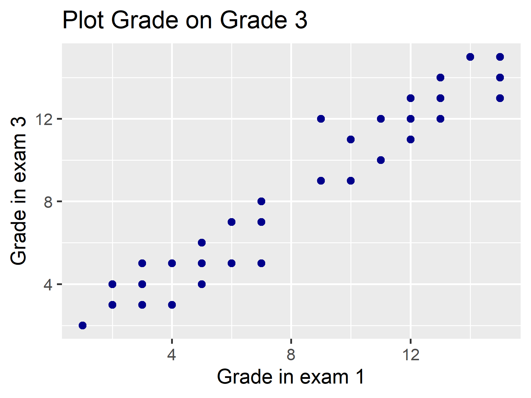
In this example, we use a fictional dataset statistics, which includes, among other things, the grade of Statistics I and the grade of Statistics II exams for students. We want to calculate a model where we determine an effect of the grade in the Statistics I exam (grade) on the grade in the Statistics II exam (grade3).
What could our theoretical assumption be for this?
We can test a linear relationship using a scatterplot. We will learn how to create this in the final learning block!
Basic Mathematics
In our example, we first calculate a bivariate linear regression:
Dependent variable:
grade3(\(y\))Independent variable:
grade(\(x_1\))
Therefore, the equation of this (bivariate) regression model is:
\(Y = \beta_0 + \beta_1 * X_1 + \varepsilon, \varepsilon \sim \mathcal{N}(0, \sigma^2)\)
\(Y\) is the dependent variable, \(X\) is the independent variable, and \(\varepsilon\) represents the residuals.
What is \(\varepsilon\) again?
And what does this expression \(\varepsilon \sim \mathcal{N}(0, \sigma^2)\) mean again?
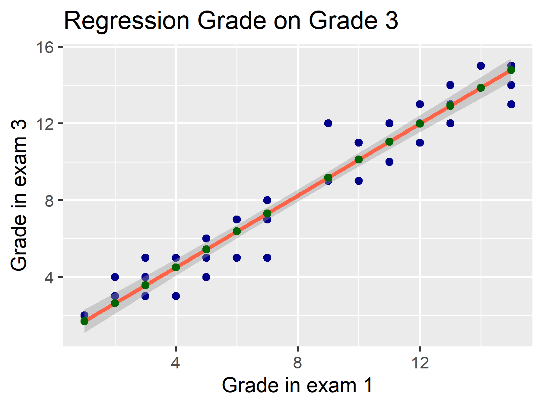
\(\varepsilon\) includes the residuals. These are the distances between the estimated value (\(\hat{y}\), green points) and the observed value (\(y\), blue points).
\(\varepsilon \sim \mathcal{N}(0, \sigma^2)\) means that these errors are normally distributed. Some residuals are positive, others negative. In total, they have a mean of \(0\) and a variance of \(\sigma^2\).
Equation of Linear Regression
Let’s briefly review the equation of linear regression:
\(Y = \beta_0 + \beta_1*X_1 + \varepsilon\)
We can also set up the equation for each case, with an index i:
\(y_i = \beta_0 + \beta_1 * {x_1}_i + \epsilon_i\)
Linear regressions are typically calculated using the Ordinary Least Squares (OLS) method. What does that mean again?
\(\sum_{i=1}^n(\hat{y_i} - y_i)^2 \to min.\)
\(\Rightarrow\) The model chooses the line that minimizes the sum of squared distances.
We can also use matrix algebra for representation. This helps (some) to better understand it in R, as we work here with vectors, matrices, and data frames (as a special form of a matrix):
\(Y = X\beta + E\)
\(\begin{bmatrix}y_1 \\y_2 \\... \\y_n \\\end{bmatrix} = \begin{bmatrix} 1 & x_1 \\ 1 & x_2 \\ 1 & ...\\ 1 & x_n\\ \end{bmatrix} \begin{bmatrix}\beta_0 \\ \beta_1\\\end{bmatrix} + \begin{bmatrix}\epsilon_1 \\ \epsilon_2 \\ ... \\ \epsilon_n \\ \end{bmatrix}\)
The model calculates the matrix \(\beta\) - in the bivariate case, two coefficients: intercept and slope of the independent variable. As a result of calculating the coefficients, we get \(E\) (residuals, the difference from observed values).
On the next page, let’s take a look at a concrete example!