Study unit 4 > Linear Regression > Bivariate Linear Regression

Bivariate Linear Regression

We are now using the dataset PSS, which we have been using throughout the exercise. We want to test how much satisfaction with economic performance explains satisfaction with democracy. The two variables you need for this linear regression are stfeco and stfdem. The theoretical premise behind this is that individuals who are economically satisfied are also more satisfied with the political system as a whole.

What is the equation for this case?

Could we also calculate a model that explains satisfaction with economic performance through satisfaction with democracy?

Yes, that’s possible! However, you would then change the theoretical assumptions here. So, you see that statistical models are not autonomous but always have a theoretical reference point!

Calculation of the Example

In R, we use the function lm() to calculate a linear regression model. It is important to know the formula because we specify the model as a formula in the function.

We store the result of the model calculation in an object! In the lm() function, you specify the formula of the linear regression in the first argument and the data object in the second argument, in this case, pss. The dataset is available in the data folder in the RStudio project. If you are working with a local version, you can download the dataset here:

Dataset

PSS_Codebook.pdf (94 KB)

pss.rds (63 KB)

olsModel <- lm(
  stfdem ~ 1 + stfeco, #Formel der Regression
  data = pss # Datenobjekt
)

In the model, we obtain various values that we need to interpret: Coefficients, t-value(or pr(>|t|)) and (adjusted) R-Squared.

The following questions should be answered at the end of each model:

How much can the model explain?
What effects do the individual variables have?

The individual values are now interpreted step by step. The results are called using the summary() function:

summary(olsModel)

## 
## Call:
## lm(formula = stfdem ~ 1 + stfeco, data = pss)
## 
## Residuals:
##     Min      1Q  Median      3Q     Max 
## -5.7171 -1.0990  0.0283  1.1556  5.7737 
## 
## Coefficients:
##             Estimate Std. Error t value Pr(>|t|)    
## (Intercept)  0.48085    0.06939    6.93 4.75e-12 ***
## stfeco       0.87271    0.01354   64.44  < 2e-16 ***
## ---
## Signif. codes:  0 '***' 0.001 '**' 0.01 '*' 0.05 '.' 0.1 ' ' 1
## 
## Residual standard error: 1.733 on 4902 degrees of freedom
##   (96 observations deleted due to missingness)
## Multiple R-squared:  0.4587,	Adjusted R-squared:  0.4585 
## F-statistic:  4153 on 1 and 4902 DF,  p-value: < 2.2e-16

Interpretation of the Coefficients

coef(olsModel)

## (Intercept)      stfeco 
##   0.4808475   0.8727124

How do we interpret the value for stfeco?

$\Rightarrow$ With each increase of one unit in stfeco, stfdem also increases by $0.8727124$ points.

$\Rightarrow$ A person with a value of $0$ in stfeco achieves a value of $0.4808475instfdem` (Intercept).

Using the confint() function, we obtain the estimated intervals (in summary() we only get the t-value and p-value):

confint(olsModel)

##                 2.5 %    97.5 %
## (Intercept) 0.3448187 0.6168763
## stfeco      0.8461641 0.8992608

In the social sciences, the interpretation of the Intercept is usually less relevant in most cases. Therefore, we primarily look at the influence of grade. The confidence interval ranges from $[0.8461641, 0.8992608]$ and does not include the value $0. This effect is therefore significant. We reject the null hypothesis that this effect is equal to $0 ($_1 =0`).

Confidence Intervals & p-Value

What do the confidence interval and the p-value tell us?

We have calculated the mean effect of stfeco on stfdem and the confidence interval of this effect.
Through significance tests (mostly t-tests), we infer that the population value ($\mu$) of this calculation is not equal to $0$ (significant p-value): It is then very unlikely ($95 %$) that $\mu = 0$.
The p-value does not allow us to say that the true value corresponds to the calculated value (e.g., with $95 %$ certainty, the true mean is within the calculated confidence interval). Because we do not know if our sample is one of the samples that includes the true value ($95 %$ of the samples include the value).
Non-significant values, therefore, tell us that we cannot rule out that the true population value ($\mu$) is equal to $0$; however, we cannot say that the true value is equal to $0$.

$\Rightarrow$ Confused? Just remember that this is about falsification and not verification (basis of empirical social research!).

Additional Output Options

If we have saved the calculation in an object, we can refer to different parts of the model (e.g., coefficients, estimated values, or residuals):

olsModel$coefficients # Koeffizienten

## (Intercept)      stfeco 
##   0.4808475   0.8727124

head(olsModel$fitted.values) # geschätzte Werte

##        1        2        3        4        5        6 
## 5.717122 6.589834 5.717122 3.971697 4.844410 5.717122

head(olsModel$residuals) # Residuen

##          1          2          3          4          5          6 
##  1.2828780  1.4101656  0.2828780  1.0283029 -0.8444096  0.2828780

We can also use the following functions instead: coef(), fitted(), resid() or confint().

coef(olsModel) # Koeffizienten

## (Intercept)      stfeco 
##   0.4808475   0.8727124

head(fitted(olsModel)) # ersten 6 geschätzten Werte

##        1        2        3        4        5        6 
## 5.717122 6.589834 5.717122 3.971697 4.844410 5.717122

head(resid(olsModel)) # Residuen

##          1          2          3          4          5          6 
##  1.2828780  1.4101656  0.2828780  1.0283029 -0.8444096  0.2828780

confint(olsModel) # Konfidenzintervalle

##                 2.5 %    97.5 %
## (Intercept) 0.3448187 0.6168763
## stfeco      0.8461641 0.8992608

Global Model Evaluation

For the global assessment of model quality, the coefficient of determination $R^2$ is often provided. $R^2$ provides information on how much of the variance of the dependent variable can be explained by the model.

The equation is:

\[R^2 = \frac{\sum_{i=1}^n(\hat{y_i}-\bar{y})^2}{\sum_{i=1}^n(y_i-\bar{y})^2} = \frac{explained \, variance}{total \, variance}\]

$R^2$

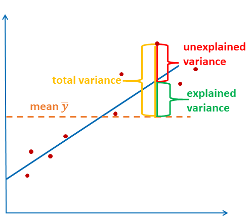
The graph illustrates the formula again: the explained variance is the sum of squared distances between estimated value and the mean. The total variance is the sum of squared distances between observed value and the mean.

How do we now describe the result? $R^2$ is given in the penultimate line.

summary(olsModel)

## 
## Call:
## lm(formula = stfdem ~ 1 + stfeco, data = pss)
## 
## Residuals:
##     Min      1Q  Median      3Q     Max 
## -5.7171 -1.0990  0.0283  1.1556  5.7737 
## 
## Coefficients:
##             Estimate Std. Error t value Pr(>|t|)    
## (Intercept)  0.48085    0.06939    6.93 4.75e-12 ***
## stfeco       0.87271    0.01354   64.44  < 2e-16 ***
## ---
## Signif. codes:  0 '***' 0.001 '**' 0.01 '*' 0.05 '.' 0.1 ' ' 1
## 
## Residual standard error: 1.733 on 4902 degrees of freedom
##   (96 observations deleted due to missingness)
## Multiple R-squared:  0.4587,	Adjusted R-squared:  0.4585 
## F-statistic:  4153 on 1 and 4902 DF,  p-value: < 2.2e-16

The model explains $45.85\%$ of the variance in satisfaction with democracy (stfdem) ($R^2$). Higher satisfaction with economic performance (stfeco) is positively associated with satisfaction with democracy (stfdem). For every one-unit increase in satisfaction with economic performance, the value of satisfaction with democracy increases by $0.87271$. The effect of stfeco on stfdem is significant ($p<0.001$).