Import of .txt and .csv
First, we will import global dataset file formats. These are .txt and .csv. For the .csv format, there is a language peculiarity. In the standard (English language version on the computer), the data delimiter is a , (comma), but on computers with German language settings, this differs, and the data delimiter is a ; (semicolon).
Importing a .txt File
A .txt file is a plain text file where data is separated by a tab (see screenshot). Here, too, the convention is that variables are entered in the columns and cases in the rows. Typically, the first row does not represent a case but contains, as in the example, the variable names.
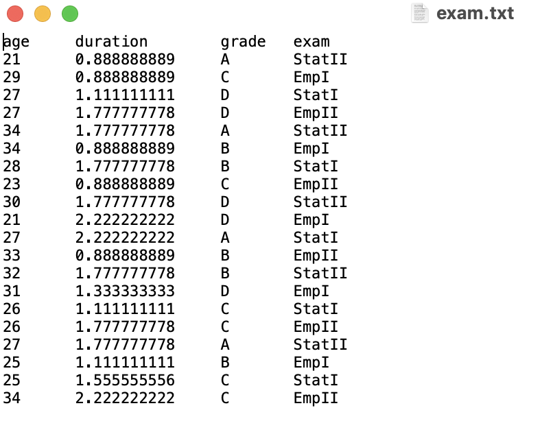 In the example, we have a dataset with four variables:
 age, duration, grade, and exam.
When you load files, you need to remember what a file path is. If you don’t remember, go back to Learning Block 1. RStudio Cloud makes this easier for us by allowing us to easily select the path: In RStudio Projects, there is always a folder named data that can be accessed as follows: ./data/, and after the second slash comes the file name. You can read about how it works with a local installation at the very bottom. However, this is not relevant for the course at the moment, as we are all working with RStudio Cloud.
In R, the Environment is where we see all the loaded and saved data and objects.
To load the .txt file (tab-separated file) in R, we need the read.table() function. Whenever you need help with a known function, you can simply put a ? in front of it and leave the arguments empty. In the Help tab in the Files pane, hints about the function will appear.
Let’s give it a try.
# If you need help with the function:
?read.table()
Now we want to import the data into R so that we can work with it. The datasets are already stored in the data folder. It’s best to name dataset objects in a way that intuitively indicates what data they contain. Within the import function (read.table()), you simply provide the full path to the file. Since the first line in the file contains the variable names, we specify header = TRUE in the last argument to indicate that the variable names are there. The argument sep = "\t" simply specifies that the delimiter for the data is a tab.
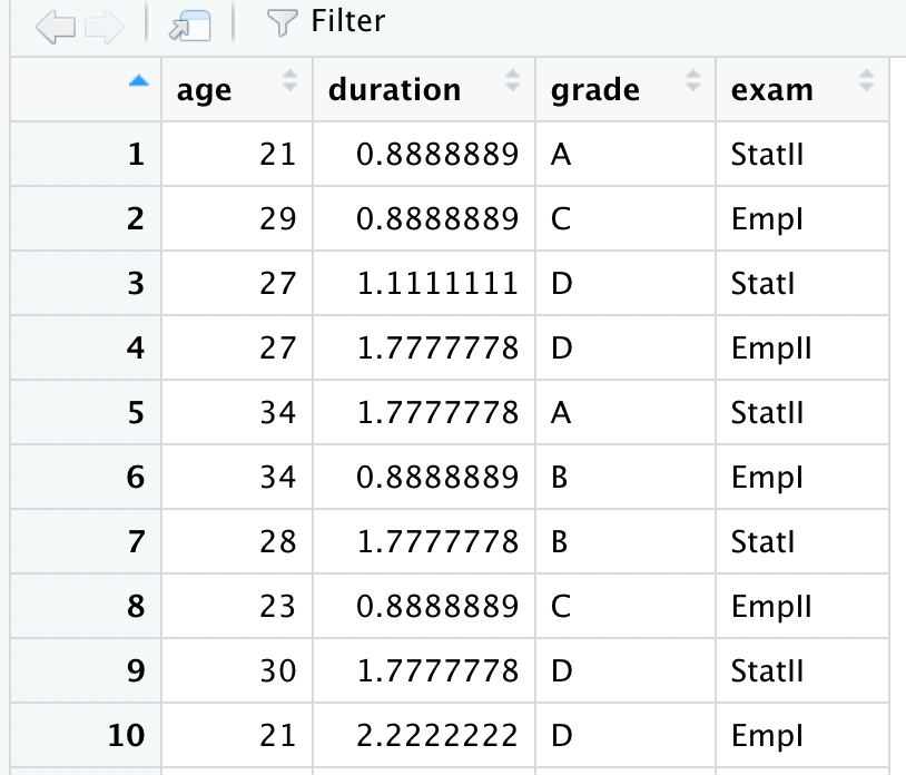
We have now imported the data and created a new data frame named exam! This is now visible in the Environment.
Structure of a Dataset
There are a number of helper functions to get an overview of imported data. You will now get to know these.
To display the structure of the dataset, you call the following function:
str(exam)## 'data.frame': 20 obs. of 4 variables:
## $ age : int 21 29 27 27 34 34 28 23 30 21 ...
## $ duration: num 0.889 0.889 1.111 1.778 1.778 ...
## $ grade : chr "A" "C" "D" "D" ...
## $ exam : chr "StatII" "EmpI" "StatI" "EmpII" ...With the function head(), we can get a first look at the data (the first \(6\) cases):
head(exam)## age duration grade exam
## 1 21 0.8888889 A StatII
## 2 29 0.8888889 C EmpI
## 3 27 1.1111111 D StatI
## 4 27 1.7777778 D EmpII
## 5 34 1.7777778 A StatII
## 6 34 0.8888889 B EmpIWe can also display more than \(6\) cases by adding a second argument specifying the number.
head(
  exam,
  n = 10   # hier kann die Anzahl verändert werden
)
## age duration grade exam
## 1 21 0.8888889 A StatII
## 2 29 0.8888889 C EmpI
## 3 27 1.1111111 D StatI
## 4 27 1.7777778 D EmpII
## 5 34 1.7777778 A StatII
## 6 34 0.8888889 B EmpI
## 7 28 1.7777778 B StatI
## 8 23 0.8888889 C EmpII
## 9 30 1.7777778 D StatII
## 10 21 2.2222222 D EmpIWe can also address individual variables within the dataset. To do this, we specify the dataset and address an individual variable using the $ sign:
head(exam$grade)## [1] "A" "C" "D" "D" "A" "B"So now you have accomplished that, and applying it to other file formats is not much more work. Next, let’s import a .csv file.
Importing a .csv file
To load a .csv file, we do not need any additional library. The function (similar to the one above) is included in R-Base.
The file includes the same dataset, just as a .csv file.
We need the function read.csv() or read.csv2(). This depends on whether you have already opened the .csv file on your computer (Excel or LibreOffice). If yes, and your computer language is German, you need to use read.csv2(). If you have never opened the file or use English language settings, use read.csv().
Let’s give it a try!
examcsv <- read.csv(
"./data/exam.csv",
header = TRUE
)
examcsv2 <- read.csv2(
"./data/exam.csv",
header = TRUE
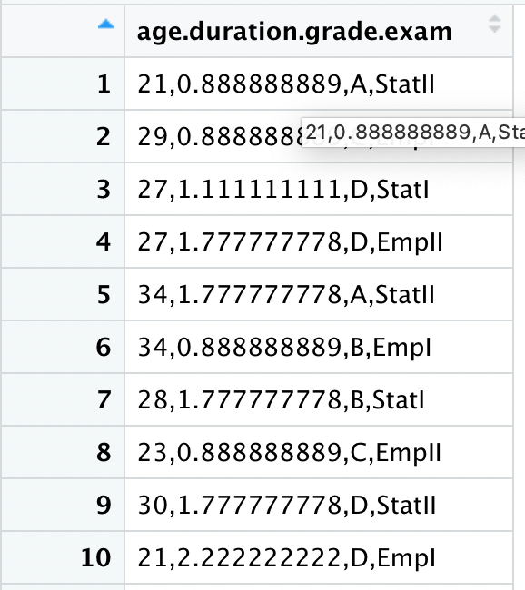
)Here you can see a screenshot of the two imported datasets using the different functions.
It is important to understand the file format and how to import it, as this can easily avoid errors during import.
Now let’s move on to the formats provided by R!
Local Work
When you work locally later on, you always have to specify the direct path of the file. Or you save the path in an object and then use this object within the helper function file.path(). The advantage is that you do not have to enter the path constantly, as it is recommended to store all datasets in one place. With this one central location, you can simply create an object containing this path as text. So, as in Learning Block 1, you simply create an object containing character that sensibly specifies the path here. This way, the path does not have to be entered anew each time.
Important: The path only goes up to the folder where the file is located. The file is not saved in the path object.
So, create an object containing the path. We usually call this path.
path <- "C:/File path to the saved object/"
# copy this from Explorer or Finder and remember to change backslashes to slashes for Windows
In the import function, you simply add the helper function file.path(), where the first argument is the object path (the character for your object) and the second argument is the file name (here exam.txt). Everything else remains as above!
exam <- read.table(
  file.path(
    path,
    "exam.txt"
  ),
  sep = "\t",
  header = TRUE
)